NOTE: This work is carried out by myself and Nitish Tongia under the supervision of Prof. Shivaram Kalyanakrishnan as course project for course CS 748 at IIT Bombay.

Monte-Carlo Exploring Starts for POMDP’s (MCESP) is a memory-less, model-free reinforcement learning algorithm that integrates the Monte Carlo exploring starts [1] into a local search of deterministic policy space to perform control tasks in partially observable Markov decision processes (POMDP’s). The novelty in this approach is the introduction of a new action-value function which ensures that the algorithm is theoretically sound and guarantees the convergence to locally optimal policies in some special cases [2]. We implement the algorithm on multiple standard partially observable domains to demonstrate the convergence properties. We then go on to modify the algorithm so that the policy search now works in the space of stochastic policies. We verify the dominance of this modified version empirically over the deterministic version and other stochastic learning algorithms in partially observable domains.

Introduction

In many realistic situations, the dynamics of the agent’s environment and observations are unknown or only partially known. In such cases, the problem of sequential decision making by intelligent agents is formulated as partially observable Markov decision processes (POMDP). The standard reinforcement learning algorithms such as Q-Learning and Sarsa(\(\lambda\)) ignore the partial observability and treat the observations as the states of a Markov decision problem (MDP). However, the theoretical soundness of such action-value based algorithms is questionable as they can fail to converge even on some very simple problems [3]. Stochastic algorithms that search through a continuous space of stochastic policies by conditioning the action choice on the agent’s immediate observation do actually converge to local optimal policies under appropriate conditions, but data suggests that the learning in these algorithms is much slower as compared to action-value based reinforcement learning algorithms.

The MCESP algorithm gets the best of both approaches by achieving the better empirical performance of the actionvalue based RL algorithms and provide stronger theoretical properties like the stochastic algorithms. It can be interpreted as a local search algorithm that achieves local optimum in the discrete space of policies that maps observation to actions. The novel action-value function in the algorithm is inspired by the work on fixed-point analysis [4]. Based on different choices of free parameters, different ideas from stochastic optimisation can be incorporated.

In model-free POMDP literature, the dominance of stochastic policy learning over deterministic policies has been heavily studied and empirically verified in a large number of independent works. In this direction, the modified version of MCESP, which we call Stochastic MCESP, performs the policy search in the space of stochastic policies. This aims to get closer and closer to the hypothetical optimum memory-less stochastic policy.

Problem Formulation

The agent’s environment is modeled as a POMDP with an unknown underlying MDP, but a finite observation set. Based on the trajectory, the agent is required to learn a deterministic policy that maximizes the discounted episodic reward under the assumption that the episodes terminate with certainty under any policy. Later, the search space of policies is extended to a much larger space of stochastic policies. There, the policy search in the continuous space is performed based on the expected value of discounted episodic reward of the trajectory under the stochastic policy.

POMDP

Partially observable markov decision process (POMDP’s) provide a generalised memory-less model for planning under uncertainty represented using \(\{S, A, O, T, \Omega, R, \gamma \}\) where \(S\) is the set of (finite) discrete states, \(A\) is the set of discrete actions, \(O\) is the set of discrete observations providing incomplete/noisy information about state, \(T(s,a,s') = Pr(s_{t+1}=s'\) | \(s_t=s, a_t=a)\) is the transition probability from state \(s\) to \(s'\) on taking action \(a\), \(\Omega(o, s, a) := Pr(o_{t+1} = o\) | \(a_t = a, s_{t+1} = s)\) is the probability of observing \(o\) from state \(s\) after taking action \(a\), \(R(s,a)\) is the reward obtained on taking action \(a\) from state \(s\) and \(\gamma\) is the discount factor.

Related Works

In partially observable domains, using standard RL algorithms which treat the observations as if they were the states of an underlying Markov decision problem (MDP) can lead to sub-optimal behaviour or in the worst case, the parameters learned by the RL algorithm can fail to converge or even diverge [5, 6]. The theoretical soundness of such algorithms is questionable if the underlying representation of the environment is not fully markov.

A large variety of algorithms which perform different kinds of stochastic gradient descent on a fixed error function have been developed [7, 8, 9]. These usually condition the action choice on immediate observation plus the state of an internal memory. Empirical evidence suggests that these are much slower than the memory-less RL algorithms because of the added complexity of storing and updating history or some sort of belief states.

The work of [2] on this MCESP algorithm differs from the general approach in this domain by defining a novel action value function which allows us to integrate exploring starts with policy search while still enjoying strong convergence properties. Our contribution of extension of the MCESP algorithm to stochastic policies and the empirical verification of its dominance over standard memory-less approaches like the work done by [10], to the best of our knowledge, is new.

MCESP

Note: Refer to Perkins 2002 [2] for more detials of deterministic MCESP.

Neighbouring Policy

One of the key aspect of MCESP algorithm is its interpretation as a local search algorithm in the space of memory-less policies. In that regard, for a policy \(\pi\), define its neighbouring policy as \(\pi \leftarrow (o, a)\) that is identical to \(\pi\) except that it assigns action \(a\) corresponding to observation \(o\).

Action Value Function

For a trajectory \(\tau\), the discounted episodic reward is defined as \(R(\tau) = \sum_{i=0}^{\infty}\gamma^ir_i\). Let an observation \(o\) occurs in trajectory \(\tau\) for the first time at time step \(j\), then we define \(R_{pre-o}(\tau) = \sum_{i=0}^{j-1}\gamma^ir_i\) and \(R_{post-o}(\tau) = \sum_{i=j}^{\infty}\gamma^ir_i\) i.e. the parts of the discounted episodic reward before and after the first occurrence of observation \(o\) respectively. Following this, we define the action value function as the expected post observation return of the neighbouring policy, i.e.

This definition of action value differs from the one in a standard MDP case in three aspects:

1. The notion of a staring state is replaced by the first occurrence of an observation \(o\)
2. After taking the immediate action \(a\), the agent follows a neighbouring policy \(\pi \leftarrow (o,a)\) of policy \(\pi\)
3. The action value function, instead of being the discounted return that follows \(o\), it is the portion of discounted reward following observation \(o\)

This definition of action value function preserves (to some degree) the property of MDP’s that an optimal is necessarily greedy with respect to its action values.

Theorem 1

For all \(\pi\) and \(\pi'=\pi \leftarrow (o,a)\)

Proof

Now, as the expected discounted reward before first occurrence of observation \(o\) is independent of the action taken from \(o \implies E^{\pi}\{R_{pre-o(\tau)}\} = E^{\pi \leftarrow (o,a)}\{R_{pre-o(\tau)}\}\)

Following these definitions, we say that a policy \(\pi\) is an \(\epsilon\) locally optimal policy if and only if its action value is at-least \(\epsilon\) beter than all its neighbouring policies, i.e. it satisfies \(Q^{\pi}_{o,\pi(o)} + \epsilon \geq Q^{\pi}_{o,a} \forall\) observations \(o\) and actions \(a\).

Algorithm

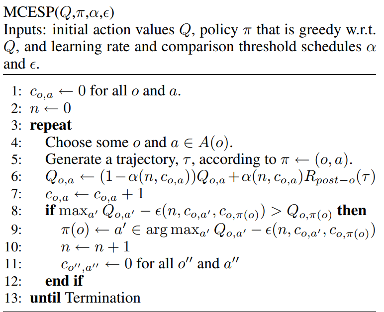
The algorithm itself can be seen as two independent parts, first between lines (4-7) and second between lines (8-12). Since the environment is only partially observable to the agent, given a policy, the action values themselves are an estimate of the true values as they are approximated using discounted reward of a finite number of trajectories. The first part of the algorithm works on bringing these action value estimates closer and closer to their true values by performing first visit Monte-Carlo updates for each selected pair of observations and actions. Based on the present estimates, the second part of the algorithm performs a policy search and tries to find neighbouring policy which is significantly better (at-least \(\epsilon\) better) than the current policy. This threshold is dependent on the number of policy updates (n) and the number of action-value updates for the selected observation-action pair (\(c_{o,a}\)) after the last policy update.

Based on different observation-action pair selection methods (uniformly at random or in round robin fashion), different learning rate schedules (\(\alpha\)) and different choices for comparison threshold (\(\epsilon\)) functions, different variants of MCSEP can be obtained which differ in their performance, computational complexity and convergence properties. We present three such variations each one of which integrate the MCESP algorithm to incorporate different ideas from stochatic optimisation literature.

MCESP SAA

If the dynamics of the POMDP are unknown to the agent, exact evaluation of any policy is not possible. By generating a fixed number of trajectories(k) under a given policy, an estimate of the policy’s value can be obtained as the average discounted return. This approach is known as Sample Average Approximation [11] in stochastic optimization literature. For larger values of k, the action-value estimates are expected to be accurate and the algorithm is expected to converge to the local-optimal solution.

\(\alpha(n,i) = \dfrac{1}{i + 1}\) and \(\epsilon(n,i,j) = \begin{cases} \infty & i < k \hspace{2mm} or \hspace{2mm} j < k \\ 0 & otherwise \end{cases}\)

MCESP PALO

In finite local neighborhood structure, PALO [12] algorithm is a general method for hill-climbing in the solution space of a stochastic optimization problem. In MCESP-PALO, the decaying learning rate corresponds to simple averaging, and the comparison threshold is based on Hoeffding’s inequality. The algorithm strictly moves towards the local optimal policy and is expected to converge with absolute certainty.

\(k_n = \left\lceil {2\dfrac{(y-x)^{2}}{\epsilon^{2}} ln\Big(\dfrac{2N}{\delta_{n}}\Big)}\right\rceil\) , \(\delta_{n} = \dfrac{6\delta}{n^{2}\pi^{2}}\) , \(\alpha(n,i) = \dfrac{1}{i + 1}\)

MCESP CE

Since the action values are stochastic, after any finite number of steps, it is not possible to achieve local optimal policy with absolute certainty. However, it serves good as an indicator of non-optimal policy and thereby suggesting a switch. This ensures that the algorithm with a constant comparison threshold will surely converge to at least a \(\epsilon\)-locally optimal policy. Here, \(\alpha(n,i) = b \times i^{-p}\) and \(\epsilon(n,i,j) = \epsilon_0\)

MCESP-SAA and MCESP-PALO are much more heavier in terms of computational complexity than MCESP-CE. So, due to resource constraints, we kept our focus on producing results for the constant-epsilon version of our algorithm. We took a couple of tasks (one episodic and one continuing) for testing the theoretical claims and verifying their correctness in general. In both of these, the state of the environment was only partially observable to the agent.

Various Partially Observable Domains

Parr and Russell’s Grid World

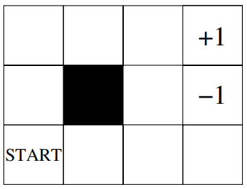
Parr and Russell’s Grid World [13] is a \(4\times 3\) grid consisting of 11 states and an obstacle state as shown in Figure 1. The environment is only partially observable to the agent as it can sense only the presence of walls to its immediate east and west and whether it is in the goal (+1) or the penalty (-1) state. The agent can take 4 actions for movement in North, South, East and West directions and its moves in the desired direction with probability 0.8 and slips to either sides with probability 0.1 each. A constant reward of -0.04 is received by the agent for each transition except for the transition to terminal states, where it receives +1 for reaching goal state and -1 for reaching penalty state. In this partially observable setting, the agent is required to learn the best memory-less policy which maximises the discounted episodic reward from the start state to the terminal state.

Chrisman’s Space Shuttle Docking Problem

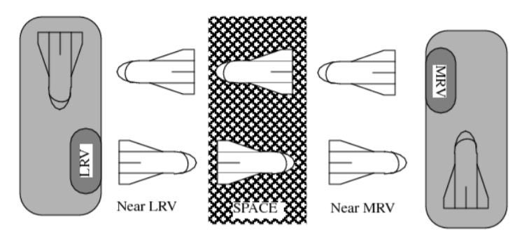
Chrisman’s Space Shuttle Docking Problem [14] comprises of two stations as shown in Figure 2. The stations are observable to the agent as least recently visited (LRV) or most recently visited (MRV) based on the most recent docking of the shuttle to one of the stations. The agent can sense only 5 different observations in this 8 state POMDP. It can observe as being in front of or being docked to one of the stations(MRV or LRV), and seeing nothing in front. Out of the three actions that agent can take, two (go-forward and turn-around) are deterministic whereas action backup succeed with probability less than 1. Action backup has different effects based on the true state of the shuttle. If the true state of the shuttle is the middle space, then action backup succeeds with probability 0.8, no effect with probability 0.1 and the effect of turn-around with probability 0.1. If the shuttle is in front of one of the stations with its back facing towards it, action backup will result in successful docking with probability 0.7 and no effect with probability 0.3. If the shuttle is already docked into one of the stations, action backup will cause the the station to deterministically change to the MRV station. If the shuttle is facing one of the stations, then action backup results in successful docking with probability 0.3, results in no effect with probability 0.4 and the effect of turn-around with probability 0.3. As the name suggests, action go-forward propels the shuttle in the forward direction and action turn-around rotates the shuttle by 180 degrees, i.e. reverse the direction of the shuttle. A reward of +10 is awarded for successful docking into the LRV (using action backup), a penalty of -3 is incurred for bumping into the station (taking action go-forward while facing the station). A constant penalty of -0.004 is incurred to incentivise the agent to perform the task as quickly as possible. The goal for the agent is to learn a memory-less deterministic policy that continuously docks to the two stations in an alternate manner.

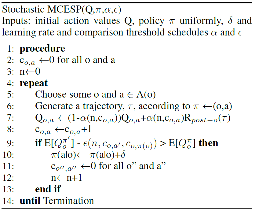
Stochastic MCESP

The dominance of stochastic policies over deterministic ones has been empirically proven in a large number of independent works and is widely accepted in pomdp literature with respect to memory-less policies. In this regard, we modified the MCESP algorithm to perform the policy search in the continuous space of stochastic policies while still maintaining the core structure of the algorithm. It differs from the deterministic version in two key aspects. First, the neighbouring policy \(\pi \leftarrow (o,a)\) is now defined on the basis of a little perturbation (\(\delta\)) in the conditional probability for an action \(a\) given an observation \(o\). And second, the policy search step is now based on the comparison between the expected values of the action value functions.

where \(\pi \leftarrow (o,a) = Normalised(\pi')\) and \(\pi'(a'|o') = \begin{cases} \hspace{10pt} \pi(a'|o') & if \hspace{7pt} (o',a') \neq (o,a)\\ \pi(a'|o')+\delta & \hspace{10pt} otherwise\\ \end{cases}\)

Results

The plots below shows the comparison between the deterministic algorithm (MCESP-CS), the stochastic algorithm (Williams and Singh [10]) and our modified algorithm (Stochastic MCESP) for Parr and Russell Grid World and Chrisman’s Shuttle problem.

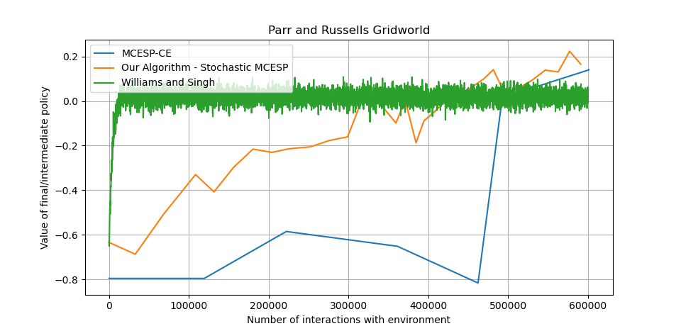
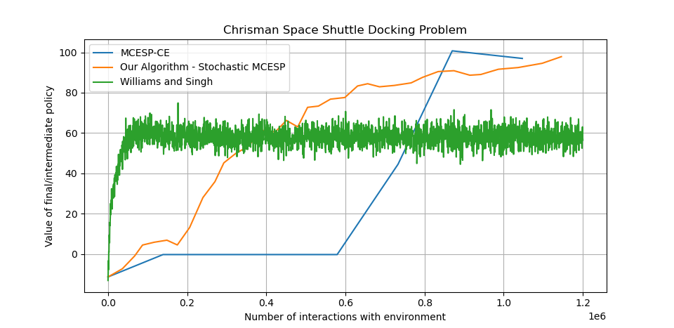
We can see from both the plots that our modified algorithm dominates both the deterministic version of MCESP and the algorithm by Williams and Singh in terms of value of the final optimal policy when restricted to same amount of training (by fixing the number of interactions with the environment). We can observe that the algorithm by Williams and Singh achieves convergence earlier, but it is nowhere near to the optimal value to which stochastic MCESP converges. Also, the amount of tuning and time taken by Willams and Singh’s is much more than by both the versions of MCESP.

Conclusion

We begin with presenting a novel algorithm MCESP, a model-free memory-less reinforcement learning algorithm for POMDP’s. We ran different variants of the algorithm on various benchmarks [15] in partially observable domains and verify the theoretical claims and convergence properties. The major drawback in our algorithm is that a lot of times, we found that the algorithm is converging to a locally and not globally optimal policy. That is the trade off that the algorithm has in order to enjoy such theoretical guarantees. We focused on one episodic and one continuous task. This can be further extended to see how these claims generalize for much more complex domains.

Since we know that memory-less stochastic policies in general work much better than deterministic ones for POMDP’s, we modified our algorithm so that now it performs the policy search in the space of stochastic policies without perturbing the core structure of the algorithm. We then compare this with the deterministic version and other stochastic learning algorithms to verify its superior performance. Still, our work is by no means completely refined in all its aspects. Several improvements might be possible like using complex strategies for exploration techniques instead of simple round-robin or selection observation-action uniformly at random.

References

1. S. Sutton, R., and G. Barto, A. 2014. Reinforcement learning: An introduction second edition: 2014, 2015.

2. Perkins, T. J. 2002. Reinforcement learning for pomdps based on action values and stochastic optimization. 199–204.

3. Gordon, G. J. 1996. Chattering in sarsa(lambda) - a cmu learning lab internal report.

4. Pendrith, M. D., and Mcgarity, M. J. 1998. An analysis of direct reinforcement learning in non-markovian domains. 421–429.

5. Whitehead, S. 1992. Reinforcement learning for the adaptive control of perception and action.

6. Baird, L. 1995. Residual algorithms: Reinforcement learning with function approximation. 30–37.

7. Williams, R. J. 1992. Simple statistical gradient-following algorithms for connectionist reinforcement learning. Machine Learning 8:229–256.

8. Baird, L., and Moore, A. 1998. Gradient descent for general reinforcement learning. 968–974.

9. Sutton, R. S.; McAllester, D. A.; Singh, S. P.; Mansour, Y.; et al. 2000. Policy gradient methods for reinforcement learning with function approximation. 99:1057–1063.

10. Williams, J. K., and Singh, S. 1999. Experimental results on learning stochastic memoryless policies for partially observable markov decision processes. 1073–1079.

11. Kleywegt, A. J.; Shapiro, A.; and Homem-de Mello, T. 2002. The sample average approximation method for stochastic discrete optimization. SIAM J. on Optimization 12(2):479–502.

12. Greiner, R. 1995. Palo: A probabilistic hillclimbing algorithm. Artificial Intelligence 83:1–2.

13. Parr, R., and Russell, S. 1995. Approximating optimal policies for partially observable stochastic domains. 95:1088–1094.

14. Chrisman, L. 1992. Reinforcement learning with perceptual aliasing: The perceptual distinctions approach. 1992:183–188

15. Cassandra, A. R. 2003. Pomdp examples. Available at pomdp.org

To cite this article:

@article{smcesp2021,
  title={Stochastic Monte Carlo Exploration Starts for POMDPs},
  author={Dahale, Rishabh and Tongia, Nitish},
  year={2021}
}